快速开始
在本例子中,我们拿 movielens
100K 来做例子。现在我们已经有三张表了,分别是pyodps_ml_100k_movies(电影相关的数据),pyodps_ml_100k_users(用户相关的数据),pyodps_ml_100k_ratings(评分有关的数据)。
如果你的运行环境没有提供 ODPS 对象,你需要自己创建该对象:
>>> import os
>>> from odps import ODPS
>>> # 保证 ALIBABA_CLOUD_ACCESS_KEY_ID 环境变量设置为用户 Access Key ID,
>>> # ALIBABA_CLOUD_ACCESS_KEY_SECRET 环境变量设置为用户 Access Key Secret
>>> # 不建议直接使用 Access Key ID / Access Key Secret 字符串
>>> o = ODPS(
...     os.getenv('ALIBABA_CLOUD_ACCESS_KEY_ID'),
...     os.getenv('ALIBABA_CLOUD_ACCESS_KEY_SECRET'),
...     project='**your-project**',
...     endpoint='**your-endpoint**',
... )
创建一个DataFrame对象十分容易,只需传入Table对象即可。
>>> from odps.df import DataFrame
>>> users = DataFrame(o.get_table('pyodps_ml_100k_users'))
我们可以通过dtypes属性来查看这个DataFrame有哪些字段,分别是什么类型
>>> users.dtypes
odps.Schema {
  user_id             int64
  age                 int64
  sex                 string
  occupation          string
  zip_code            string
}
通过head方法,我们能取前N条数据,这让我们能快速预览数据。
>>> users.head(10)
   user_id  age  sex     occupation  zip_code
0        1   24    M     technician     85711
1        2   53    F          other     94043
2        3   23    M         writer     32067
3        4   24    M     technician     43537
4        5   33    F          other     15213
5        6   42    M      executive     98101
6        7   57    M  administrator     91344
7        8   36    M  administrator     05201
8        9   29    M        student     01002
9       10   53    M         lawyer     90703
有时候,我们并不需要都看到所有字段,我们可以从中筛选出一部分。
>>> users[['user_id', 'age']].head(5)
   user_id  age
0        1   24
1        2   53
2        3   23
3        4   24
4        5   33
有时候我们只是排除个别字段。
>>> users.exclude('zip_code', 'age').head(5)
   user_id  sex  occupation
0        1    M  technician
1        2    F       other
2        3    M      writer
3        4    M  technician
4        5    F       other
又或者,排除掉一些字段的同时,得通过计算得到一些新的列,比如我想将sex为M的置为True,否则为False,并取名叫sex_bool。
>>> users.select(users.exclude('zip_code', 'sex'), sex_bool=users.sex == 'M').head(5)
   user_id  age  occupation  sex_bool
0        1   24  technician      True
1        2   53       other     False
2        3   23      writer      True
3        4   24  technician      True
4        5   33       other     False
现在,让我们看看年龄在20到25岁之间的人有多少个
>>> users[users.age.between(20, 25)].count()
195
接下来,我们看看男女用户分别有多少。
>>> users.groupby(users.sex).agg(count=users.count())
   sex  count
0    F    273
1    M    670
用户按职业划分,从高到底,人数最多的前10职业是哪些呢?
>>> df = users.groupby('occupation').agg(count=users['occupation'].count())
>>> df.sort(df['count'], ascending=False)[:10]
      occupation  count
0        student    196
1          other    105
2       educator     95
3  administrator     79
4       engineer     67
5     programmer     66
6      librarian     51
7         writer     45
8      executive     32
9      scientist     31
DataFrame API提供了value_counts这个方法来快速达到同样的目的。注意该方法返回的行数受到 options.df.odps.sort.limit
的限制,详见 配置选项 。
>>> uses.occupation.value_counts()[:10]
      occupation  count
0        student    196
1          other    105
2       educator     95
3  administrator     79
4       engineer     67
5     programmer     66
6      librarian     51
7         writer     45
8      executive     32
9      scientist     31
让我们用更直观的图来看这份数据。
>>> %matplotlib inline
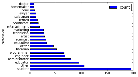
我们可以用个横向的柱状图来可视化
>>> users['occupation'].value_counts().plot(kind='barh', x='occupation', ylabel='prefession')
<matplotlib.axes._subplots.AxesSubplot at 0x10653cfd0>
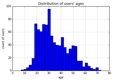
我们将年龄分成30组,来看个年龄分布的直方图
>>> users.age.hist(bins=30, title="Distribution of users' ages", xlabel='age', ylabel='count of users')
<matplotlib.axes._subplots.AxesSubplot at 0x10667a510>
好了,现在我们把这三张表联合起来,只需要使用join就可以了。join完成后我们把它保存成一张新的表。
>>> movies = DataFrame(o.get_table('pyodps_ml_100k_movies'))
>>> ratings = DataFrame(o.get_table('pyodps_ml_100k_ratings'))
>>>
>>> o.delete_table('pyodps_ml_100k_lens', if_exists=True)
>>> lens = movies.join(ratings).join(users).persist('pyodps_ml_100k_lens')
>>>
>>> lens.dtypes
odps.Schema {
  movie_id                            int64
  title                               string
  release_date                        string
  video_release_date                  string
  imdb_url                            string
  user_id                             int64
  rating                              int64
  unix_timestamp                      int64
  age                                 int64
  sex                                 string
  occupation                          string
  zip_code                            string
}
现在我们把年龄分成从0到80岁,分成8个年龄段,
>>> labels = ['0-9', '10-19', '20-29', '30-39', '40-49', '50-59', '60-69', '70-79']
>>> cut_lens = lens[lens, lens.age.cut(range(0, 81, 10), right=False, labels=labels).rename('年龄分组')]
我们取分组和年龄唯一的前10条看看。
>>> cut_lens['年龄分组', 'age'].distinct()[:10]
   年龄分组  age
0       0-9    7
1     10-19   10
2     10-19   11
3     10-19   13
4     10-19   14
5     10-19   15
6     10-19   16
7     10-19   17
8     10-19   18
9     10-19   19
最后,我们来看看在各个年龄分组下,用户的评分总数和评分均值分别是多少。
>>> cut_lens.groupby('年龄分组').agg(cut_lens.rating.count().rename('评分总数'), cut_lens.rating.mean().rename('评分均值'))
     年龄分组  评分均值  评分总数
0       0-9  3.767442        43
1     10-19  3.486126      8181
2     20-29  3.467333     39535
3     30-39  3.554444     25696
4     40-49  3.591772     15021
5     50-59  3.635800      8704
6     60-69  3.648875      2623
7     70-79  3.649746       197