Quick start
Here, movielens 100K is used as an example. Assume that three tables already exist, which are pyodps_ml_100k_movies (movie-related data), pyodps_ml_100k_users (user-related data), and pyodps_ml_100k_ratings (rating-related data).
Create a MaxCompute object before starting the following steps:
>>> import os
>>> from odps import ODPS
# Make sure environment variable ALIBABA_CLOUD_ACCESS_KEY_ID already set to Access Key ID of user
# while environment variable ALIBABA_CLOUD_ACCESS_KEY_SECRET set to Access Key Secret of user.
# Not recommended to hardcode Access Key ID or Access Key Secret in your code.
>>> o = ODPS(
...     os.getenv('ALIBABA_CLOUD_ACCESS_KEY_ID'),
...     os.getenv('ALIBABA_CLOUD_ACCESS_KEY_SECRET'),
...     project='**your-project**',
...     endpoint='**your-endpoint**',
... )
You only need to input a Table object to create a DataFrame object. For example:
>>> from odps.df import DataFrame
>>> users = DataFrame(o.get_table('pyodps_ml_100k_users'))
View fields of DataFrame and the types of the fields through the dtypes attribute, as shown in the following code:
>>> users.dtypes
odps.Schema {
  user_id             int64
  age                 int64
  sex                 string
  occupation          string
  zip_code            string
}
You can use the head method to obtain the first N data records for easy and quick data preview. For example:
>>> users.head(10)
   user_id  age  sex     occupation  zip_code
0        1   24    M     technician     85711
1        2   53    F          other     94043
2        3   23    M         writer     32067
3        4   24    M     technician     43537
4        5   33    F          other     15213
5        6   42    M      executive     98101
6        7   57    M  administrator     91344
7        8   36    M  administrator     05201
8        9   29    M        student     01002
9       10   53    M         lawyer     90703
You can add a filter on the fields if you do not want to view all of them. For example:
>>> users[['user_id', 'age']].head(5)
   user_id  age
0        1   24
1        2   53
2        3   23
3        4   24
4        5   33
You can also exclude several fields. For example:
>>> users.exclude('zip_code', 'age').head(5)
   user_id  sex  occupation
0        1    M  technician
1        2    F       other
2        3    M      writer
3        4    M  technician
4        5    F       other
When excluding some fields, you may want to obtain new columns through computation. For example, add the sex_bool attribute and set it to True if sex is Male. Otherwise, set it to False. For example:
>>> users.select(users.exclude('zip_code', 'sex'), sex_bool=users.sex == 'M').head(5)
   user_id  age  occupation  sex_bool
0        1   24  technician      True
1        2   53       other     False
2        3   23      writer      True
3        4   24  technician      True
4        5   33       other     False
Obtain the number of persons at age of 20 to 25, as shown in the following code:
>>> users[users.age.between(20, 25)].count()
195
Obtain the numbers of male and female users, as shown in the following code:
>>> users.groupby(users.sex).agg(count=users.count())
   sex  count
0    F    273
1    M    670
To divide users by job, obtain the first 10 jobs that have the largest population, and sort the jobs in the descending order of population. See the following:
>>> df = users.groupby('occupation').agg(count=users['occupation'].count())
>>> df.sort(df['count'], ascending=False)[:10]
      occupation  count
0        student    196
1          other    105
2       educator     95
3  administrator     79
4       engineer     67
5     programmer     66
6      librarian     51
7         writer     45
8      executive     32
9      scientist     31
DataFrame APIs provide the value_counts method to quickly achieve the same result. An example is shown below. Note that the number of records returned by this method is limited by options.df.odps.sort.limit, whose default value is 10,000. More information can be found in configuration section.
>>> uses.occupation.value_counts()[:10]
      occupation  count
0        student    196
1          other    105
2       educator     95
3  administrator     79
4       engineer     67
5     programmer     66
6      librarian     51
7         writer     45
8      executive     32
9      scientist     31
Show data in a more intuitive graph, as shown in the following code:
>>> %matplotlib inline
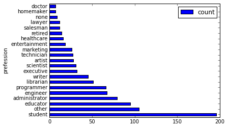
Use a horizontal bar chart to visualize data, as shown in the following code:
>>> users['occupation'].value_counts().plot(kind='barh', x='occupation', ylabel='prefession')
<matplotlib.axes._subplots.AxesSubplot at 0x10653cfd0>
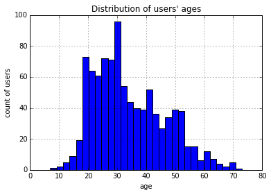
Divide ages into 30 groups and view the histogram of age distribution, as shown in the following code:
>>> users.age.hist(bins=30, title="Distribution of users' ages", xlabel='age', ylabel='count of users')
<matplotlib.axes._subplots.AxesSubplot at 0x10667a510>
Use join to join the three tables and save the joined tables as a new table. For example:
>>> movies = DataFrame(o.get_table('pyodps_ml_100k_movies'))
>>> ratings = DataFrame(o.get_table('pyodps_ml_100k_ratings'))
>>>
>>> o.delete_table('pyodps_ml_100k_lens', if_exists=True)
>>> lens = movies.join(ratings).join(users).persist('pyodps_ml_100k_lens')
>>>
>>> lens.dtypes
odps.Schema {
  movie_id                            int64
  title                               string
  release_date                        string
  video_release_date                  string
  imdb_url                            string
  user_id                             int64
  rating                              int64
  unix_timestamp                      int64
  age                                 int64
  sex                                 string
  occupation                          string
  zip_code                            string
}
Divide ages of 0 to 80 into eight groups, as shown in the following code:
>>> labels = ['0-9', '10-19', '20-29', '30-39', '40-49', '50-59', '60-69', '70-79']
>>> cut_lens = lens[lens, lens.age.cut(range(0, 81, 10), right=False, labels=labels).rename('age_group')]
View the first 10 data records of a single age in a group, as shown in the following code:
>>> cut_lens['age_group', 'age'].distinct()[:10]
   age_group  age
0        0-9    7
1      10-19   10
2      10-19   11
3      10-19   13
4      10-19   14
5      10-19   15
6      10-19   16
7      10-19   17
8      10-19   18
9      10-19   19
View users’ total rating and average rating of each age group, as shown in the following code:
>>> cut_lens.groupby('age_group').agg(cut_lens.rating.count().rename('total_rating'), cut_lens.rating.mean().rename('avg_rating'))
     age_group  avg_rating  total_rating
0          0-9    3.767442            43
1        10-19    3.486126          8181
2        20-29    3.467333         39535
3        30-39    3.554444         25696
4        40-49    3.591772         15021
5        50-59    3.635800          8704
6        60-69    3.648875          2623
7        70-79    3.649746           197